How To Combine Two Data Sets In Excel

When most people use PivotTables, they copy the source data into a worksheet, then deport out a lot of VLOOKUPs to become the categorization columns into the information set. Later that, the data is ready, nosotros tin can create a PivotTable, and the assay tin start. But we don't need to do all those VLOOKUPs anymore. Instead, we can build relationships that combine multiple tables and automatically create the lookups for u.s..

We don't need to copy and paste data into some other worksheet either as we can now use Power Query to import the information. Check out my Ability Query serial to empathize how to do this. For this post, we are focusing on creating relationships.

The ability to create relationships has been around since Excel 2022, yet many users don't even know this feature exists.

Download the example file

I recommend you download the example file for this post. Then you'll be able to piece of work along with examples and meet the solution in activeness, plus the file will be useful for future reference.

Download the file: 0040 Combining multiple tables in a PivotTable.zip

Spotter the video

Watch the video on YouTube.

The scenario

In our example file, we have three sections of information:

Sales data
Sales rep data
Product data

Sections of data for Pivot Table

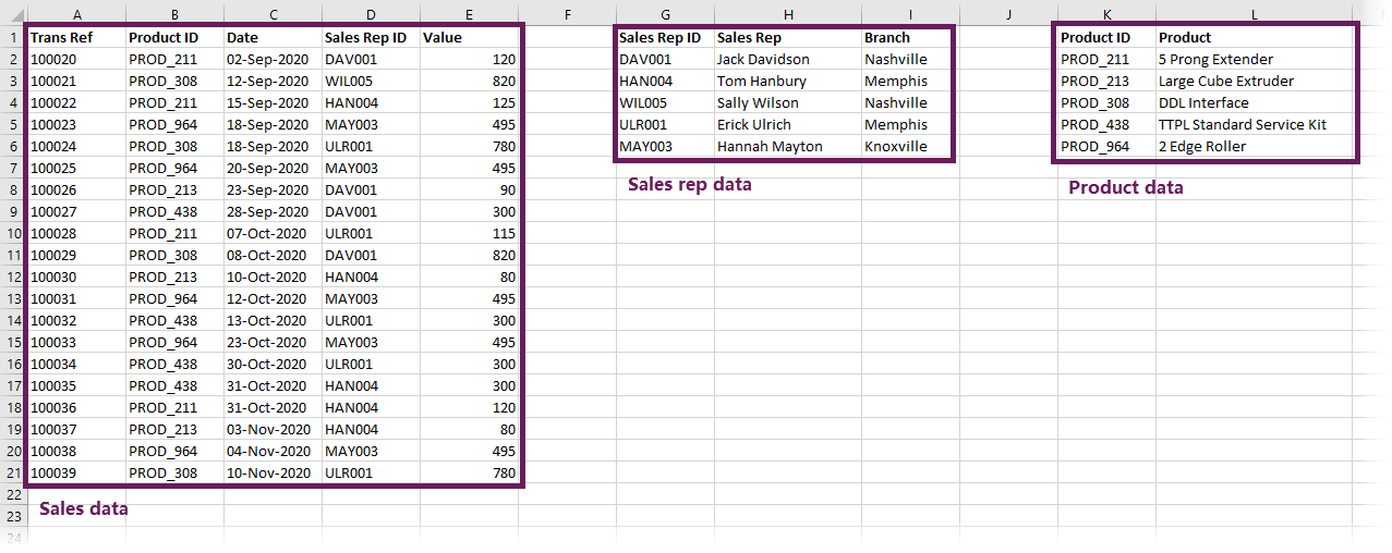
These data sets could exist on dissever worksheets, merely for ease of sit-in, I take included them on i.

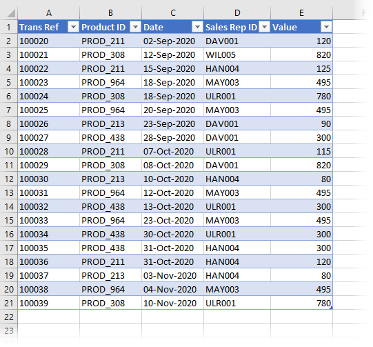
The sales data contains the transaction information, which is often referred to equally a fact table. The sales rep data and product data include the categorization to analyze the transactions by; these are often referred to every bit lookup tables.

Our goal is to create a PivotTable showing production sales by branch; this requires information from all iii data tables. To achieve this, we are going to create relationships and volition not use a single formula!

PivotTable with relationshiops

Create tables

First, we need to turn our data into Excel tables. This puts our data into a container then that Excel knows that information technology'southward in a structured format that tin can be used to create relationships.

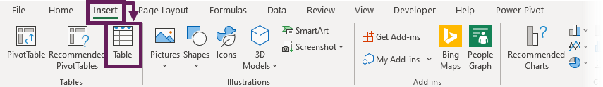
Select on whatsoever cell in the first cake of data and click Insert > Tabular array (or press Ctrl + T).

Insert - Table from Ribbon

The Create Table dialog box opens. Check the range encompasses all the information, and ensure my data has headers is ticked. Then click OK

Create table dialog box

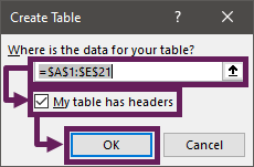
The data will change to a striped format. This is a visual indicator that an Excel tabular array has been created.

Data converted to Table

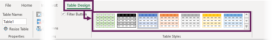
Yous don't need to stick with that format. Click any cell in the table, then click Tabular array Design and choose another format from those available.

Select Table Format

Next, with whatever jail cell in the tabular array selected, click Tabular array Design > Table Name and requite the table a meaningful name. I've called SalesData (spaces and almost special characters are not permitted within tabular array names).

Table Design - Name Table

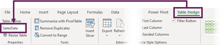
Repeat the steps above for the other datasets to create tables called SalesRepData and ProductData.

Creating relationships

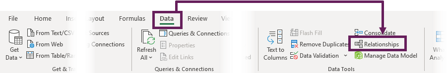
With our 3 tables created, information technology's at present time to outset creating the relationships. Click Data > Relationships.

Data - Relationships

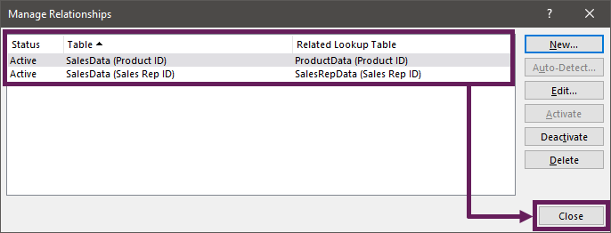
The Manage Relationships dialog box opens. Click New.

Manage Relationships - New

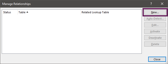
Now the Create Relationship dialog box opens. This is where nosotros ascertain the relationships that exist.

Create Relationship Window

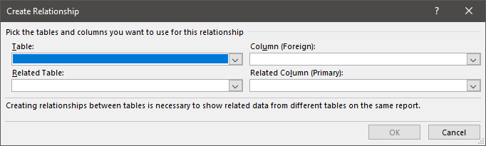
I don't remember the descriptions in this dialog box are particularly clear, so I'll effort to give you a fleck of a steer.

Table: This is the table containing the transactional values that we want to analyze (the fact table).
Column (Foreign): This is the proper name of the column from the transactional values table which we want to lookup from. If you're in the VLOOKUP mindset, then this would exist the cavalcade containing the lookup_value argument. The give-and-take Foreign is database terminology to indicate that this column can accept duplicate values.
Related table: This is the table containing the categories we want to analyze the transactional data by (the lookup table).
Related Column (Primary): This is the cavalcade nosotros want to pair with the Cavalcade (Foreign) nosotros selected above. If this were a VLOOKUP, it would exist the first column in the table_array argument. The word Principal is database terminology again; information technology tells united states that the column must contain unique values.

The columns do non need to share a mutual header for this technique to work. All the same, it tin can be helpful to remember how the tables are related.

In our example, we use the following:

Tabular array: SalesData
Column (Strange): Sales Rep ID
Related Table: SalesRepData
Related Column (Primary): Sales Rep ID

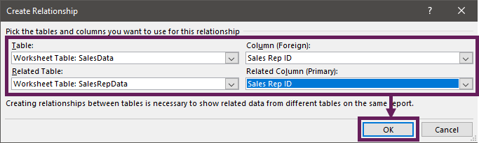
Create Relationship - Populated for Example

Click OK to create the relationship.

Now permit'southward create the relationship between the SalesData and ProductData tables using the same process as in a higher place.

Tabular array: SalesData
Column (Foreign): Production ID
Related Table: ProductData
Related Column (Primary): Product ID

Create Relationship for 2nd Table

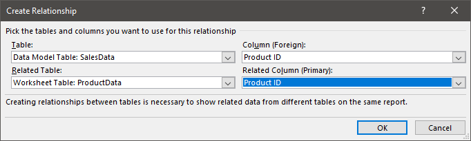
Once all the relationships are created, click Close.

Create the PivotTable

Everything is in place, so we're now set to create our PivotTable.

Click Insert > PivotTable from the ribbon.

The Create PivotTable window opens. The about important thing is that the Use this workbook's Information Model option is selected.

Create PivotTables

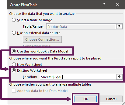
Select a location where the PivotTable should be created. For this example, we will make the PivotTable on the same worksheet equally the data. I've selected the Existing Worksheet in cell G10, but you can put your Pivot Table wherever you like.

Click OK.

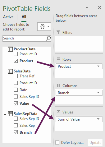
The PivotTable is created. Notice that the PivotTable Fields window includes all 3 tables. We tin can now kickoff dragging fields from each table to form a single view.

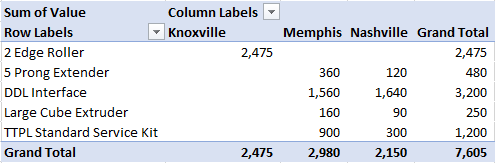
As I said earlier, the goal is to show product sales past branch. To achieve this, put the fields into the following sections:

Columns: SalesRepData > Co-operative
Rows: ProductData > Production
Values: SalesData > Sum of Value

If y'all don't see all the tables in the PivotTable Fields view, then modify the selection from Active to All.

PivotTable Fields

This creates the post-obit PivotTable:

PivotTable with relationshiops

There you take information technology. We've created a PivotTable from multiple tables without any formulas 🙂

Duplicate values in lookup tables

If we have duplicate values in our lookup tables (or related tables as they are called in the Relationships window), the relationships won't work. When we apply VLOOKUP, Excel always returns the commencement item it finds, fifty-fifty if it'south not the answer we want). Simply when we use relationships, if in that location is more than one, Excel doesn't know which detail to use; therefore, to ensure the integrity of our data, we must have unique values in our lookup tables.

Creating a human relationship with duplicate values

When creating the relationship, if we have duplicate values in our lookup tabular array, we will get the following fault:

Duplicate values when creating relationships

Nosotros must go dorsum and fix our source table before we create the relationship.

Adding duplicate values into a tabular array?

If we accidentally add duplicate values into our lookup tables, we will get an fault when refreshing the PivotTable.

Error message when duplicating values

We must go back and fix the data in the lookup table and so refresh once again.

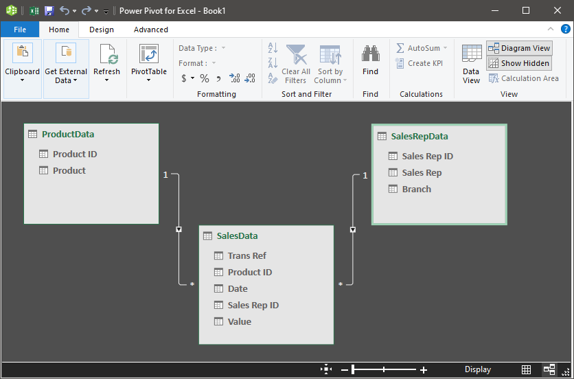
Power Pivot

You lot probably didn't realize, only you've just used the Power Pivot engine in Excel. We've not opened or installed the Power Pivot add together-in; all nosotros've used is the standard Excel interface. However, if we were to open the Power Pivot tool, we would see that our data and relationships exist in in that location.

PowerPivot - Data Model

Conclusion

In this post, we've created a PivotTable from dissever tables without formulas, something which was not possible earlier Excel 2022.

If you sympathize how these relationships work, maybe it's time to investigate Power Pivot a scrap further. Then you can gain even more automation benefits and create even more advanced reports.

Go our FREE VBA eBook of the 30 well-nigh useful Excel VBA macros.

Automate Excel and then that you can save fourth dimension and stop doing the jobs a trained monkey could do.

Claim your free eBook

Don't forget:

If yous've found this post useful, or if you have a better approach, then please leave a annotate below.

Practice you demand help adapting this to your needs?

I'one thousand guessing the examples in this mail didn't exactly see your situation. We all use Excel differently, so it'due south impossible to write a post that volition run into everybody's needs. By taking the time to understand the techniques and principles in this post (and elsewhere on this site) you should exist able to adapt it to your needs.

Only, if you're withal struggling you should:

Read other blogs, or watch YouTube videos on the aforementioned topic. You will benefit much more by discovering your own solutions.
Enquire the 'Excel Ninja' in your role. Information technology's astonishing what things other people know.
Inquire a question in a forum similar Mr Excel, or the Microsoft Answers Community. Remember, the people on these forums are by and large giving their fourth dimension for free. So take care to craft your question, make sure it's clear and concise. List all the things you've tried, and provide screenshots, code segments and example workbooks.
Use Excel Rescue, who are my consultancy partner. They assist by providing solutions to smaller Excel problems.

What next?
Don't go yet, in that location is plenty more than to acquire on Excel Off The Grid. Check out the latest posts: